Recently, a bunch of us in NCBS began to dabble in machine learning and artificial neural networks (ANN). We even created our own journal club to discuss papers on the cutting edge of machine-learning and began implementing them ourselves. We started by writing our own libraries in order to gain a deeper understanding of the math behind ANNs (you can look at our libraries here). Having done this, we finally decided to begin using TensorFlow as it provided us with a set of efficient (…better written) libraries which we can use to work on real-world projects.
Our first order of business was to run through all the tutorials in TensorFlow, starting with the beginner’s mnist tutorial. We realized that the TensorFlow documentation is slightly obscure, hence this blog (/Jupyter notebook). The beginner’s mnist is essentially a linear model and therefore simply implements a perceptron. Surprisingly, a simple perceptron gives a nice classification accuracy of 92%.
import tensorflow as tf
%matplotlib inline
import matplotlib.pyplot as plt
import matplotlib.image as mpimg
import numpy as np
import seaborn as sns
sns.set(color_codes=True)

from tensorflow.examples.tutorials.mnist import input_data
mnist = input_data.read_data_sets("MNIST_data/", one_hot=True)
The first few lines import TensorFlow and other necessary libraries for reshaping and plotting images. The last line downloads and loads the mnist dataset (read_data_sets does this automatically). mnist is now an object with training, test and validation data nicely sorted. mnist.train.images, for example, contains all the training images. Each image is 28x28 and linearized into a vector of size 784 (28x28). There are 55000 such training images, making the size of the training set (55000, 784). To look at the images, one has to extract and reshape them, as shown below.
np.shape(mnist.train.images)(55000, 784)
plt.imshow(np.reshape(mnist.train.images[0,:],[28,28]), cmap='Greys')
Sample image from the mnist dataset
The labels for each training image is stored as a ‘one-hot vector’. This essentially means there are 9 columns of output for each image (each row in mnist.train.images),
mnist.train.labels[0,:]array([ 0., 0., 0., 0., 0., 0., 0., 1., 0., 0.])
Let’s now train a perceptron for the mnist classification task. We can easily do this by writing the perceptron as a simple linear classifier. The input x, which is our image, has a dimension of [image_number, 784]. This is a 2D matrix with each image as a row with 784 columns (28x28). Because the number of images is variable and depends on the training batch size, we use a placeholder to create it. Inputs are mostly created using placeholders as one of the dimensions (number of images trained) is generally variable. The weight is essentially is [784, 10] matrix which transforms each image into a one-hot vector. The bias is an intercept for each output and is therefore a vector of size 10 (bias sets the classification threshold of each output). The classification output therefore will have a dimension of [image_number, 10]. Essentially, the set of equations can be imagined as a perceptron as shown below.
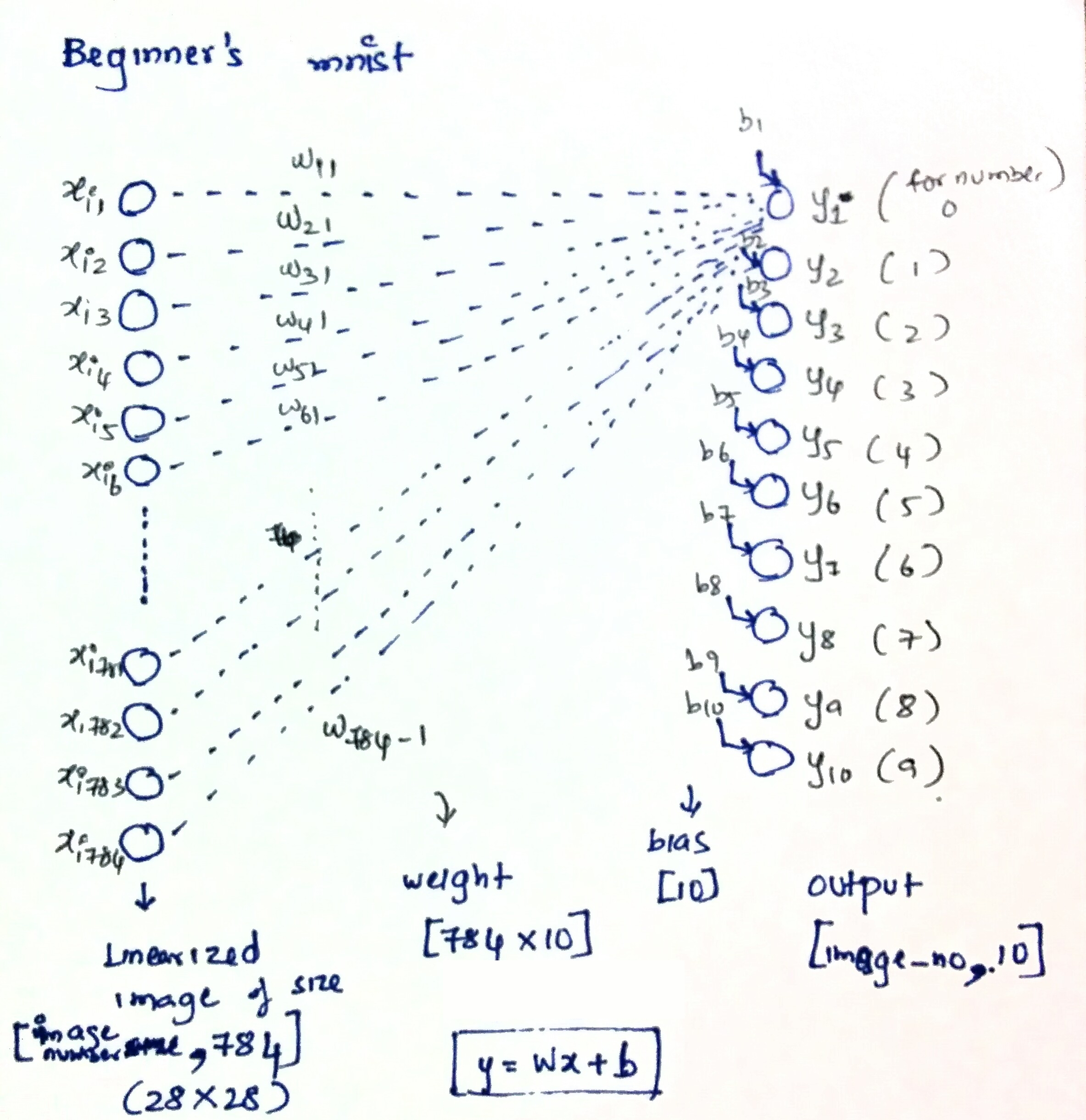
Visualization and equations for the perceptron (/linear classifier)
The next step is to convert the output into probabilities (very useful). One simple way of doing this is to softmax the output. The softmax function is a multinomial generalization of a logistic regression (generally used for categorical distributions). A simple logistic regression essentially converts an independent variable into the probability of obtaining a binary dependent variable which can take only two values - “0” or “1”. Softmax (a.k.a Multinomial Logistic_regression) takes in multiple independent variables and converts it into probabilities of a categorical distribution (i.e. it gives a probability of obtaining one of (n) input variables). This is convenient as it ensures that the sum of the output is always one (thereby valid probabilities).
Once the output is classified, we have to compare the output classification with the ground truth and change the weights depending on it. There are a couple of ways of doing it. One simple way is the mean squared distance (or the L2 distance). Another (complicated but better) loss function is cross-entropy. There are several advantages of using cross-entropy over mean squared distance (nicely demonstrated in this blog post). Minimizing cross-entropy is same as minimizing Kullback-Leibler divergence, which is essentially the distance (information gain) of the obtained probability distribution and the true probability distribution (in bits). If both of them are same, which is true for perfect classification, then KL divergence goes to zero. Minimizing KL or cross-entropy by backpropagating the error is therefore one way of training the perceptron.
# Input and weights
x = tf.placeholder(tf.float32, [None, 784])
W = tf.Variable(tf.zeros([784, 10]))
b = tf.Variable(tf.zeros([10]))

# Output (apply softmax)
y_o = tf.nn.softmax(tf.matmul(x, W) + b)

# Cross entropy (loss function)
y_ = tf.placeholder(tf.float32, [None, 10])   # The ground truth (one-hot vectors)
y = tf.matmul(x, W) + b
cross_entropy = tf.reduce_mean(
      tf.nn.softmax_cross_entropy_with_logits(labels=y_, logits=y))

# Add train step
train_step = tf.train.GradientDescentOptimizer(0.5).minimize(cross_entropy)
In the code above, instead of applying the softmax function to the output and then computing the cross-entropy, TensorFlow recommends applying softmax_cross_entropy_with_logits. This essentially ensures that multinomial logistic regression is applied properly on the output (carefully covering numerical instabilities) before finding the cross entropy (read more on this here). The final line puts everything together by defining the train step with a learning rate and the loss function.
The below set of codes trains and tests the perceptron, giving a test accuracy of approx 92%.
# Create a session and train
sess = tf.InteractiveSession()
tf.global_variables_initializer().run()
# Train
for _ in range(1000):
    batch_xs, batch_ys = mnist.train.next_batch(100)
    sess.run(train_step, feed_dict={x: batch_xs, y_: batch_ys})
# Test trained model
correct_prediction = tf.equal(tf.argmax(y, 1), tf.argmax(y_, 1))
accuracy = tf.reduce_mean(tf.cast(correct_prediction, tf.float32))
print(sess.run(accuracy, feed_dict={x: mnist.test.images,
y_: mnist.test.labels}))0.9195
It is more fun to visualize the trained weights which provide intuition of how the perceptron classifies the mnist data. The weights are shown as images below.
fig, ax = plt.subplots(nrows=2, ncols=5)
fig.set_size_inches(18.5, 10.5)


for i in range(10):
    ax[int(i/5)][int(i%5)].imshow(np.reshape(W[:,i].eval(),[28,28]))
Weights (W) for each output node (i.e. digit) of the perceptron
The weights (shown above) seems to encapsulate each number more or less accurately. Numbers 0, 1, 2, 3 are more or less apparent (red is positive weights and blue is negative). The other numbers are a bit harder to visualize from the weights. Numbers 4, 5, 8 and 9 are the least apparent (atleast to me). Does the apparency of the weights in the images above somehow predict the accuracy of the classifications? That is, does the perceptron perform badly for the numbers 4, 5, 8 and 9?
To answer this, I simply plotted the errors for each digit classification and plotted the histogram below. The least apparent weights to in fact have a lot more classification errors (except for 4). Maybe the errors are due to incomplete learning of the weights. Or maybe the the errors are because of multiple representation of the error prone digits causing a blurred learning of both. Either way, a deep network should do even better on the dataset thereby giving better classification. I will try out the deep mnist tutorial next and blog about it soon!
prediction = tf.equal(tf.argmax(y, 1), tf.argmax(y_, 1))
classifications = sess.run(prediction, feed_dict={x: mnist.test.images, y_: mnist.test.labels})
_, labels = np.nonzero(mnist.test.labels)
incorrect_classified = [labels[i] for i, p in enumerate(classifications) if not p]np.shape(incorrect_classified)(816,)
sns.distplot(incorrect_classified, bins=20, kde=False, rug=True)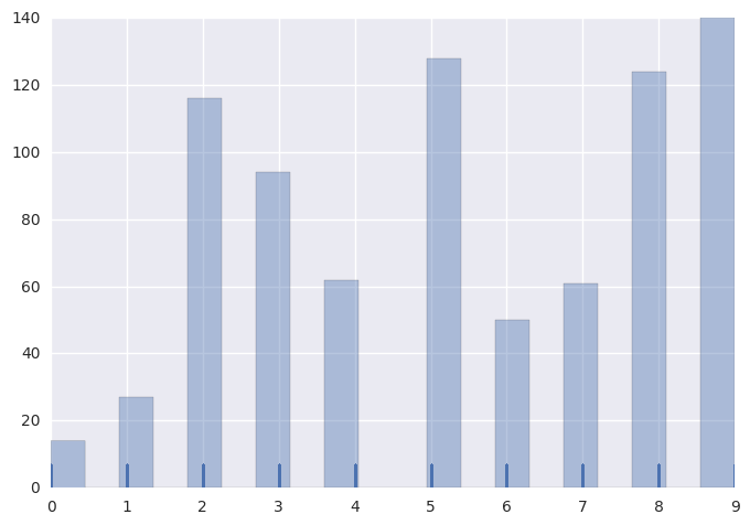
Histogram of incorrectly classified digits by the perceptron