Cross-correlation between two timeseries

Cross-correlation is conceptually is actually quite simple, but it often gets masked behind its mathy definition. So instead of focusing on math, I will try to illustrate this concept numerically (inspired by Statistical rethinking).

Let’s start by defining cross-correlation. Cross-correlation is a measure of how two signals change in time. If two signals increase and decrease together - they are correlated in time. If one signal increases and the other decreases - they are anti-correlated. And if changes in one is independent from the other - they are uncorrelated.

The “cross” in correlation just refers to cross-talk between two signals, causing a correlation in time. The problem with time varying signals is that there is often delays - two signals can be correlated but one can be delayed with respect to the other causing it to seem uncorrelated or anti-correlated. With cross-correlation, we can also measure how the correlation between signals changes by artificially adding delays to figure out if one signal is just a delayed version of the other.

In the first section, we will establish the concept of quantifying cross-correlation between two signals. Then, we will extend this concept to computing correlation for different delays between two signals.

Concept

To simply things, let’s find the correlation between two sine waves. The idea of cross-correlation is simple - to figure out if two signals are correlated, all we need to do is multiple them and take the area under the curve (AUC) of the resulting signal.

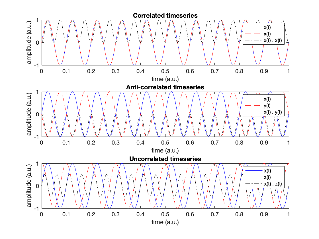
There are three scenarios for the sine waves (and for any signal):

1. Both of them are moving together (correlated, top) - the multiplication will be positive giving rise to a positive area under the curve.
2. Both of them are moving exactly opposite (anti-correlated, middle) - the multiplication will be negative giving rise to a negative area under the curve.
3. Both of them are moving independently (uncorrelated, bottom) - the multiplication will be positive sometimes and negative sometimes. Overall the area under the curve will be almost zero.

Code

MATLAB

% Cross-correlation between two timeseries
% Concept
 
t = 0:0.001:1; % 0-1 sec, 1kHz sampling rate
f = 10; % Hz
 
x = sin(2*pi*f*t);
y = -1 * x;
z = cos(2*pi*f*t);
 
% figure
figure(1);
 
title('Correlated timeseries');
subplot(3,1,1), plot(t,x,'-b');
hold on, plot(t,x,'--r');
hold on, plot(t, x .* x, '-.k');
legend({'x(t)', 'x(t)', 'x(t) . x(t)'});
xlabel('time (a.u.)');
ylabel('amplitude (a.u.)');
 
title('Anti-correlated timeseries');
subplot(3,1,2), plot(t,x,'-b');
hold on, plot(t,y,'--r');
hold on, plot(t, x .* y, '-.k');
legend({'x(t)', 'y(t)', 'x(t) . y(t)'});
xlabel('time (a.u.)');
ylabel('amplitude (a.u.)');
 
title('Uncorrelated timeseries');
subplot(3,1,3), plot(t,x,'-b');
hold on, plot(t,z,'--r');
hold on, plot(t, x .* z, '-.k');
legend({'x(t)', 'z(t)', 'x(t) . z(t)'});
xlabel('time (a.u.)');
ylabel('amplitude (a.u.)');

Now, the problem with just calculating area, is that it will keep increasing as the length of the signal increases. So, we need to normalize it somehow so that we know when two signals are perfectly correlated, perfectly anti-correlated or uncorrelated.

One way of normalizing it is using the best case scenarios - which is when both signals are the same. If we do that, we will get the correlation coefficient to be 1 when the signals are the correlated, -1 when the signals are anti-correlated and 0 when the signals are uncorrelated.

So, if we use this logic, we can define cross-correlation for two signals $a(t)$ and $b(t)$ as:¹

$$R_{xy}=\frac{AUC(a(t).b(t))}{\sqrt{AUC(a(t).a(t)).AUC(b(t).b(t))}}$$

To measure AUC, we can simply take the mean² of the signal:³

$$R_{xy}=\frac{E[a(t).b(t)]}{\sqrt{E[a(t).a(t)].E[b(t).b(t)]}}$$

So, when we do this for the three scenarios, this is what we get:

1. $R_{xx}=\frac{0.5}{\sqrt{0.5.0.5}}=1$
2. $R_{xy}=\frac{-0.5}{\sqrt{0.5.0.5}}=-1$
3. $R_{xz}=\frac{-0.0}{\sqrt{0.5.0.5}}=0$

Code

MATLAB

% calculate
fprintf('E[x(t) . x(t)] = %0.2f\n', mean(x .* x));
fprintf('E[x(t) . y(t)] = %0.2f\n', mean(x .* y));
fprintf('E[y(t) . y(t)] = %0.2f\n', mean(y .* y));
fprintf('E[x(t) . z(t)] = %0.2f\n', mean(x .* z));
fprintf('E[z(t) . z(t)] = %0.2f\n', mean(z .* z));

Incorporating delay

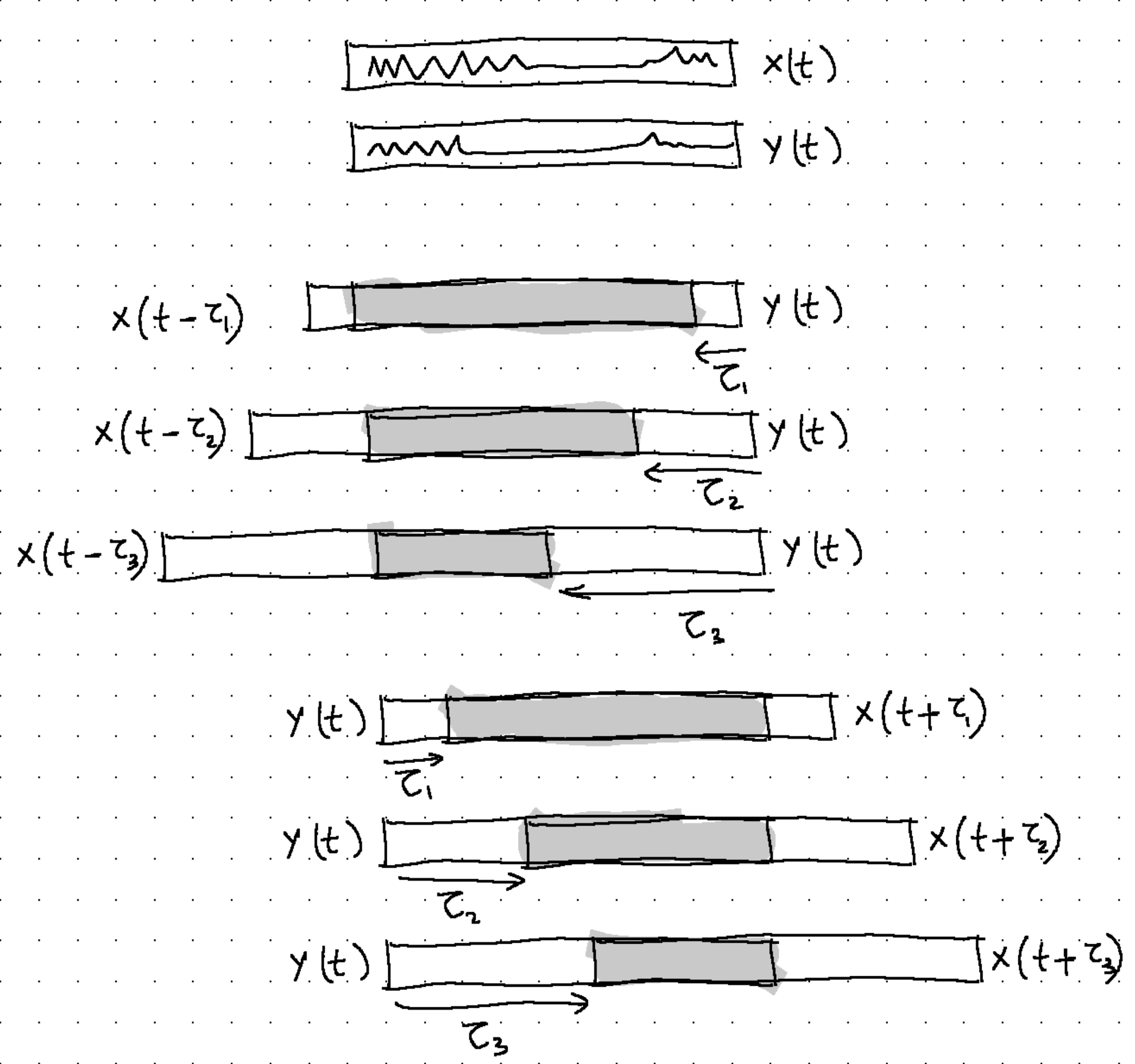
Often, in real systems, two signals might be correlated, but they are separated by a finite delay. In our example above, if the sine waves were delayed by a small amount, we could call them correlated. So in addition to just finding the cross-correlation at the current time, we should shift them slightly to see if they are correlated at any time.

This is sort of a weird thing to do because we lose data points when we shift them. So we shouldn’t do too much as the point of cross-correlation of a time series loses meaning if we shift it completely.⁴

Each shift gives us one cross-correlation value, that is dependent on the shift. We will have to be careful to prune the signals after the shift so that the signal lengths match appropriately for the multiplication.⁵ We can write this as:

$$\begin{array}{rl}{R}_{xy}(\tau )& =\frac{E[a(t-\tau ).b(t)]}{\sqrt{E[a(t-\tau ).a(t-\tau )].E[b(t).b(t)]}}\end{array}$$

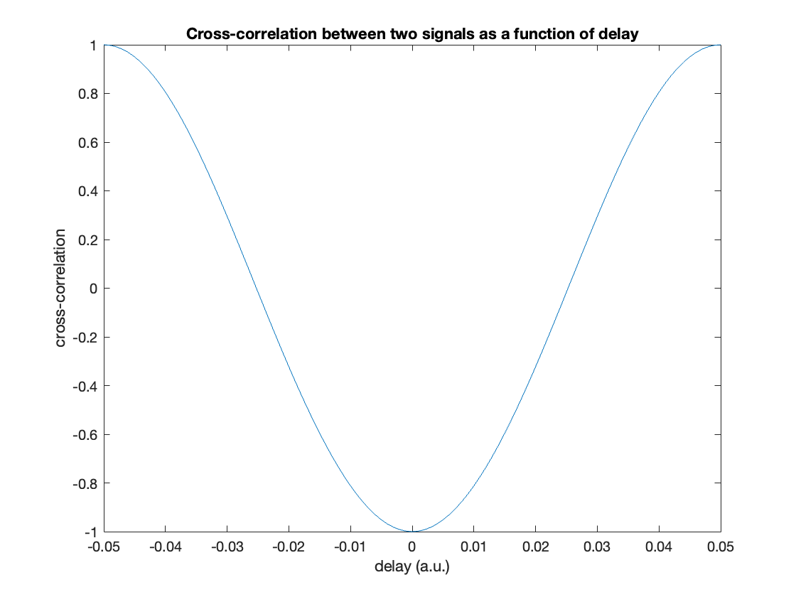
Once we calculate the cross-correlation for all our delays in our range, we can plot it to see if there any peak in correlation or anti-correlation at any particular delays.

Code

MATLAB

% Incorporating delay
data_length = length(t); % 1001
corr_neg_tau = nan(floor(data_length/20),1); % 250
corr_pos_tau = nan(floor(data_length/20),1); % 250
 
for tau=1:data_length/20
 
	% left shift x(t) - positive tau
	x_sh = x(tau+1:end); % shift x by tau
	y_pru = y(1:end-tau); % prune y by tau
	corr_neg_tau(tau) = mean(x_sh .* y_pru) /...
		sqrt(mean(x_sh .* x_sh) * mean(y_pru .* y_pru));
	
	% right shift x(t) - positive tau
	x_sh = x(1:end-tau); % shift x by tau
	y_pru = y(tau+1:end);
	corr_pos_tau(tau) = mean(x_sh .* y_pru) /...
		sqrt(mean(x_sh .* x_sh) * mean(y_pru .* y_pru));
 
end
 
% get tau for zero
corr_tau_zero = mean(x .* y) /...
	sqrt(mean(x .* x) * mean(y .* y));
 
% put them in the right order
delay = -0.05:0.001:0.05;
cross_corr = [corr_neg_tau(end:-1:1); corr_tau_zero; corr_pos_tau];
 
figure(2);
title('Cross-correlation between two signals as a function of delay');
plot(delay, cross_corr)
xlim([-0.05, 0.05]);
ylim([-1,1]);
xlabel('delay (a.u.)');
ylabel('cross-correlation');

Because our signals are sinusoids of period 0.1, I used a maximum time delay of 0.05. If we shift x by half a period (0.05), it will be y and will be correlated. If we shift x by 1/4 a period (0.025), then it will be z and will be uncorrelated.

Summary

Cross-correlations are useful to figure out if two signals increase or decrease together.

One of the most important use cases for cross-correlations is to figure out if two signals are correlated but one is delayed with respect to the other. Examples⁶ of use-cases include:

• Neuroscience: Activity of neuron 1 being correlated to neuron 2, but being delayed by an amount. This can happen if neuron 1 controls the activity of neuron 2, but change in activity of neuron 2 happens after a delay.
• Stock market: If changes in stock 1 are correlated with stock 2 but delayed by a certain amount. If they are correlated, there are possible cause-and-effect relationships between the two.

For these examples, the signals are very complicated and the cross-correlation will tell us at which delays two signals are maximally correlated.

Footnotes

1. We actually have two signals $a(t)$ and $b(t)$, so we cannot just use the best case scenario for one - we have to use both and take its square root. If we do this, when $a(t)=b(t)$ then the cross-correlation coefficient comes out to 1. ↩

2. Also called expected value of the signal and is denoted by $E[\dots ]$ ↩

3. This is not technically accurate, but it works because we are normalizing it by the mean of the original signals. We could also simply sum the signals, and that would work too (much closer to the AUC). Going with mean because that is the convention. ↩

4. How much we should shift depends a lot on the data and what makes sense for the type of data. Matlab, by default, shifts till there is only 1 value overlap between the signal, which might not make sense always (or maybe even most of the time). ↩

5. There are multiple ways to do it. One easy way is to pad it with zeros and just make sure to pick the same vector size, but offset by the time delay. The zeros won’t affect the calculation and we can do it much faster than pruning. I will prune it, just for fun. ↩

6. I will add more examples as I think of them. ↩