Geocentric models & Gaussian models

I really like the introduction about Ptolemy! I never did think about it too deeply, especially the comparison of epicycles to the Fourier series - no wonder he could fit any planetary movement time series. The fact that he sort of got it a millennia before Fourier and as able to fit it without a computer is indeed impressive.

“These days, when scientists wish to mock someone, they might compare him to a supporter of the geocentric model. But Ptolemy was a genius. His mathematical model of the motions of the planets (Figure 4.1) was extremely accurate. To achieve its accuracy, it employed a device known as an epicycle, a circle on a circle. It is even possible to have epiepicycles, circles on circles on circles. With enough epicycles in the right places, Ptolemy’s model could predict planetary motion with great accuracy. And so the model was utilized for over a thousand years. And Ptolemy and people like him worked it all out without the aid of a computer. Anyone should be flattered to be compared to Ptolemy.” (McElreath, 2020, p. 71)

“Given enough circles embedded in enough places, the Ptolemaic strategy is the same as a Fourier series, a way of decomposing a periodic function (like an orbit) into a series of sine and cosine functions. So no matter the actual arrangement of planets and moons, a geocentric model can be built to describe their paths against the night sky.” (McElreath, 2020, p. 71)

And I quite like the analogy of linear regression as geocentric models of applied statistics! That is, it fits the data really well and provides accurate predictions, while being mechanistically wrong (like the geocentric models). It is useful to use linear regression as long as we remember not to make mechanistic inferences from the model.

The 2023 video (this one) goes a bit more how Gauss invented linear regression (Bayesian approach) with gaussian (measurement) error and least-squares estimation.

Normal distributions

Normal by addition

The author gives a good intuition of why taking sums of distributions will give rise to a normal distribution.

“Here’s a conceptual way to think of the process. Whatever the average value of the source distribution, each sample from it can be thought of as a fluctuation from that average value. When we begin to add these fluctuations together, they also begin to cancel one another out. A large positive fluctuation will cancel a large negative one. The more terms in the sum, the more chances for each fluctuation to be canceled by another, or by a series of smaller ones in the opposite direction. So eventually the most likely sum, in the sense that there are the most ways to realize it, will be a sum in which every fluctuation is canceled by another, a sum of zero (relative to the mean)” (McElreath, 2020, p. 73)

For fun, I delved a bit deeper into the Central limit theorem (CLT) that provides a stronger form of this statement. It says that if a sequence of random variables $\{X_1,X_2,\dots ,X_{n-1},X_n\}$ are sampled from a distribution with mean $\mu$ and variance ${\sigma }^2$, and we compute the sample average ${\bar{X}}_n$, then the sample average distribution will be a gaussian distribution with mean $\mu$ and sigma $\frac{{\sigma }^2}{n}$ .

I tried applying this to the random walk on the soccer field example from the book. I replaced the uniform distribution with a binomial distribution to mimic steps towards left (-1) or right (+1). I expect the mean and variance for the distribution to be 0 and 1 respectively.¹

# binomial distribution 
pos <- replicate(100,  {function (x) (1*x + -1*(1-x))}(rbinom(1,1,0.5)))
library(rethinking)
dens(pos)
mean(pos)![[Garden/resource-notes/courses/Bayesian Statistics/attachments/Pasted image 20240213134403.png]]ge of 100 coin tosses (and replicating it 10000) times, gives the below distribution.  
![[Garden/resource-notes/courses/Bayesian Statistics/attachments/Pasted image 20240213134403.png]]
 
```R
# sampling
pos <- replicate(10000,  {function (x,y) (1*x + -1*(y-x))/y}(rbinom(1,100,0.5), 100))
dens(pos)
mean(pos)
variance(pos)
variance(sqrt(100)*(pos-mean(pos)))

The mean comes out to be 0, as expected. And the variance comes out to be ~0.01, which is $\frac{1}{\sqrt{n}}$, with $n=100$ as we have averaged over 100 tosses.² So as expected from CLT, the distribution of the mean of random variables from a binomial distribution has a mean of mean $\mu$ and sigma $\frac{{\sigma }^2}{n}$.

Normal by multiplication

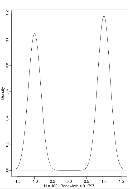
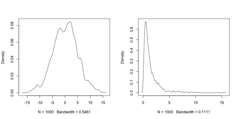
This was initially surprising as I figured multiplication would not produce Gaussian distributions. Turns out, it does for small effect multiplication. Basically, this is because multiplication of small effects can be approximated as a linear effect (the author describes this nicely in the book). For large effects, it gives rise to log-normal distribution.

In a sense, multiplication gives rise to log-normal distributions. For low-effect multiplications, log-normal distribution approximate to normal distributions.

This is cool because log-normal distributions are seen often in data. In fact, we see it in our angular velocities (and, I think, speeds) of flies tracking odor (this paper), but we did not include it as we did not quite understand what it mean. Based on this, I guess this implies that angular velocity (and speed) control might arise due to some multiplicative effects of control? Not sure, but this is an interesting concept to think about.

Why use Gaussian distributions as a default model?

The author provides a couple of convincing reasons:

“Measurement errors, variations in growth, and the velocities of molecules all tend towards Gaussian distributions. These processes do this because at their heart, these processes add together fluctuations.” (McElreath, 2020, p. 75)

“The Gaussian is a member of a family of fundamental natural distributions known as the exponential family. All of the members of this family are important for working science, because they populate our world.” (McElreath, 2020, p. 75)

“This epistemological justification is premised on information theory and maximum entropy.” (McElreath, 2020, p. 76)

Basically, same as the idea of the geocentric models, a variable does not need to be normally distributed for the gaussian model to be useful. Given the above justifications, any natural additive or a small effect multiplicative process is going to be approximately gaussian, but even if it is not, using the mean/variance for approximating the variable is a useful way of thinking about the variable distribution. It is a good default (least assumption) model to start with.

That said, the author provides a cautionary note about using Gaussian distribution as the default data model as there are cases where it will fail completely.

“Gaussian distribution has some very thin tails—there is very little probability in them. Instead most of the mass in the Gaussian lies within one standard deviation of the mean. Many natural (and unnatural) processes have much heavier tails. These processes have much higher probabilities of producing extreme events. A real and important example is financial time series—the ups and downs of a stock market can look Gaussian in the short term, but over medium and long periods, extreme shocks make the Gaussian model (and anyone who uses it) look foolish.” (McElreath, 2020, p. 76)

An example is stable distributions, which have heavy tails. This was discussed often in the CSHL Neural Data summer school I attended - in heavy tail distributions extreme events have non-zero probabilities making its occurrence possible over long periods (unlike Gaussian distributions).

Probability density vs mass

This is something that confused me often in the past. Probability density of functions can often give rise to values about 1 (like dnorm(0,0,0.01)). But since probabilities should sum up to one, why even get densities greater than 1? It took me a while to get that area under the curve of the probability density functions is what should sum up to 1. The density can be greater than 1, but it might have a shorter interval making the area under the curve small. Effectively, it is like saying that a rectangle with 1x1 and a 4x0.25 both have an area of 1. Having areas with y value = 4 just means that the probability is concentrated over fewer random variables. Most of the confusion came from going from binomial distributions where they are described by probability mass functions to gaussian (and other continuous) distribution where they were described by probability density functions, without clear distinction between them. The author does a good job providing distinctions in the book.

“Probability distributions with only discrete outcomes, like the binomial, are called probability mass functions and denoted Pr. Continuous ones like the Gaussian are called probability density functions, denoted with p or just plain old f, depending upon author and tradition.”

“Probability density is the rate of change in cumulative probability. So where cumulative probability is increasing rapidly, density can easily exceed 1. But if we calculate the area under the density function, it will never exceed 1. Such areas are also called probability mass.” (McElreath, 2020, p. 76)

Language for describing models

The general approach for description is:

“(1) First, we recognize a set of variables to work with. Some of these variables are observable. We call these data. Others are unobservable things like rates and averages. We call these parameters.
(2) We define each variable either in terms of the other variables or in terms of a probability distribution.
(3) The combination of variables and their probability distributions defines a joint generative model that can be used both to simulate hypothetical observations as well as analyze real ones.” (McElreath, 2020, p. 77)

This approach applied to the globe tossing model:

1. Variables and parameters:
   • (Variable) W: Observed count of water
   • (Variable) N: Total number of tosses
   • (Parameter)p: proportion of water
2. Define variables and parameters in terms of other variables or a probability distribution $$\begin{array}{rl}W& \sim Binomial(N,p)\\ p& \sim Uniform(0,1)\end{array}$$
3. Based on this, we can come up with our posterior distributions (and predictive posterior distribution) which can be used to simulate and analyze data
   $Pr(p|w,n)=\frac{Binomial(w|n,p)Uniform(p|0,1)}{\int Binomial(w|n,p)Uniform(p|0,1)}$

Gaussian model of height

An example of applying the language and models to the height distribution in the Howell database. The distribution of height looks like this:

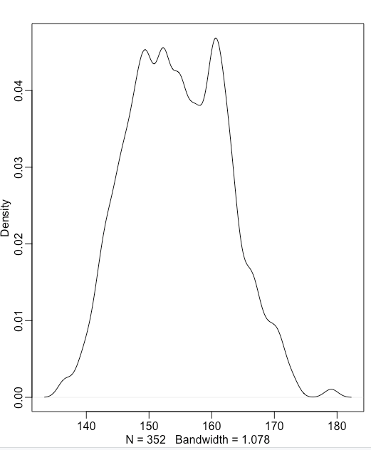
x-axis units: cm; y-axis: density

A simple model is to assume that the heights are normally distributed with some mean ($\mu$) and some standard deviation ($\sigma$). We can assume some reasonable priors for $\mu$ and $\sigma$, and come up with a model.

The model we fit is:

$$\begin{array}{rl}{h}_i& \sim Normal(\mu ,\sigma )\\ \mu & \sim Normal(178,20)\\ \sigma & \sim Uniform(0,50)\end{array}$$

Most of this section (and the corresponding code) is fitting this model using grid approximation) and quadratic approximation and visualizing the data.

Here are some key quotes from the section.

“But be careful about choosing the Gaussian distribution only when the plotted outcome variable looks Gaussian to you. Gawking at the raw data, to try to decide how to model them, is usually not a good idea. The data could be a mixture of different Gaussian distributions, for example, and in that case you won’t be able to detect the underlying normality just by eyeballing the outcome distribution. Furthermore, as mentioned earlier in this chapter, the empirical distribution needn’t be actually Gaussian in order to justify using a Gaussian probability distribution.” (McElreath, 2020, p. 81)

“The prior predictive simulation is an essential part of your modeling. Once you’ve chosen priors for h, μ, and σ, these imply a joint prior distribution of individual heights. By simulating from this distribution, you can see what your choices imply about observable height. This helps you diagnose bad choices.” (McElreath, 2020, p. 82)

“In this case, we have so much data that the silly prior is harmless. But that won’t always be the case. There are plenty of inference problems for which the data alone are not sufficient, no matter how numerous. Bayes lets us proceed in these cases. But only if we use our scientific knowledge to construct sensible priors. Using scientific knowledge to build priors is not cheating. The important thing is that your prior not be based on the values in the data, but only on what you know about the data before you see it.” (McElreath, 2020, p. 84)

The last quote gave rise to this thought about weak priors when there is no previous data about priors.

“The jargon “marginal” here means “averaging over the other parameters.”” (McElreath, 2020, p. 86)

“The 5.5% and 94.5% quantiles are percentile interval boundaries, corresponding to an 89% compatibility interval. Why 89%? It’s just the default. It displays a quite wide interval, so it shows a high-probability range of parameter values. If you want another interval, such as the conventional and mindless 95%, you can use precis(m4.1,prob=0.95). But I don’t recommend 95% intervals, because readers will have a hard time not viewing them as significance tests. 89 is also a prime number, so if someone asks you to justify it, you can stare at them meaningfully and incant, “Because it is prime.” That’s no worse justification than the conventional justification for 95%.” (McElreath, 2020, p. 88)

Linear prediction

Building model and estimating priors

The goal here is to fit a linear regression model to predict the height of an individual from their weight. The data looks like this:

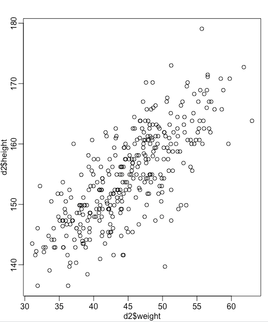
Traditionally, this what we would do:

$$h_i=m.w_i+c$$

$m$ would be the slope of the lne. c would be the intercept. And the linear regression would fit the best line (that minimizes the residuals) for this data.

Instead, we can model the height as a Gaussian with its mean dependent on the weight of the individual. This would provide us with distributions for height, as well as the slope and the intercept.

$$\begin{array}{rl}{h}_i& \sim Normal({\mu }_i,\sigma )\\ {\mu }_i& =c+m.w_i\end{array}$$

In this definition, interpretation of $c$ is a bit tricky. $w_i$ has a non-zero mean, so both the intercept needs to account for it. However, if we subtract out the mean, the interpretation becomes easier.

$$\begin{array}{rl}{h}_i& \sim Normal({\mu }_i,\sigma )\\ {\mu }_i& =\alpha +\beta .(w_i-\bar{w})\end{array}$$

Now, $\alpha$ contains the mean height of an individual, and $\beta$ contains the conversion of weight to height for the different between the individual weight and the mean weight. From here it is clear that $m=\beta$ but $c=\alpha +\beta .\bar{w}$, making its interpretation dependent on $\beta$. Subtracting the mean from the predictor therefore makes the variables easy to interpret (and setup priors).

The prior for $\alpha$ is easy - it is the average height of the distribution and we can set it as the same as the prior for the Gaussian height exercise. The prior for $\beta$ is tricker as we don’t know a reasonable conversion between weight to height. The idea is to test out a wide range and then narrow down on a window that makes sense. In the book, the window that makes sense is the size of the embryo (0) to the tallest man (~275 cm).To find out what prior makes sense, we can just setup distributions of $\alpha$ and $\beta$ and see how the lines look like with respect to the window.

One of the first things we see is that setting up $\beta$ as a normal distribution implies that we get a scenario where $\beta$ is negative - that is the height decreases when the weight is more than the average. Because we already account for the variability in height ($\sigma$), this shouldn’t happen - $\beta$ should always be positive. One way of setting this is make the $\beta$ a log-normal distribution.

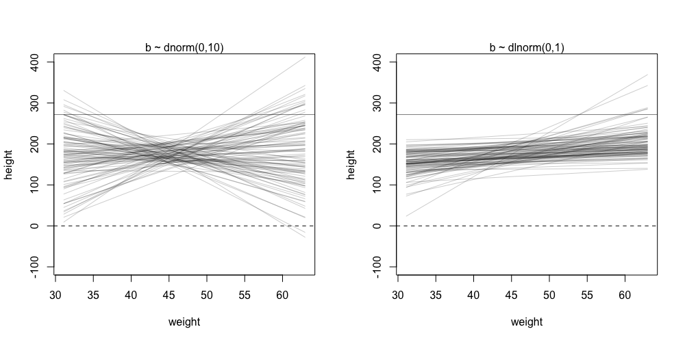
“This is the reason that Log-Normal priors are commonplace. They are an easy way to enforce positive relationships.” (McElreath, 2020, p. 96)

Importance of setting reasonable priors:

“We’re fussing about this prior, even though as you’ll see in the next section there is so much data in this example that the priors end up not mattering. We fuss for two reasons. First, there are many analyses in which no amount of data makes the prior irrelevant. In such cases, non-Bayesian procedures are no better off. They also depend upon structural features of the model. Paying careful attention to those features is essential. Second, thinking about the priors helps us develop better models, maybe even eventually going beyond geocentrism.” (McElreath, 2020, p. 96)

“Making choices tends to make novices nervous. There’s an illusion sometimes that default procedures are more objective than procedures that require user choice, such as choosing priors. If that’s true, then all “objective” means is that everyone does the same thing. It carries no guarantees of realism or accuracy.” (McElreath, 2020, p. 97)

Importance of using pre-data and not real data to choice priors:

“Prior predictive simulation and p-hacking: A serious problem in contemporary applied statistics is “p-hacking,” the practice of adjusting the model and the data to achieve a desired result. The desired result is usually a p-value less then 5%. The problem is that when the model is adjusted in light of the observed data, then p-values no longer retain their original meaning. False results are to be expected. We don’t pay any attention to p-values in this book. But the danger remains, if we choose our priors conditional on the observed sample, just to get some desired result. The procedure we’ve performed in this chapter is to choose priors conditional on pre-data knowledge of the variables their constraints, ranges, and theoretical relationships. This is why the actual data are not shown in the earlier section. We are judging our priors against general facts, not the sample. We’ll look at how the model performs against the real data next.” (McElreath, 2020, p. 97)

Finding the posterior distribution

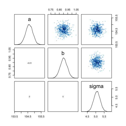
After estimating reasonable priors, the model comes out to be:

$$\begin{array}{rl}{h}_i& \sim Normal({\mu }_i,\sigma )\\ {\mu }_i& =\alpha +\beta .(w_i-\bar{w})\\ \alpha & \sim Normal(178,20)\\ \beta & \sim LogNormal(0,1)\\ \sigma & \sim Uniform(0,50)\end{array}$$

Fitting a linear model onto the dataset provides us with the following distribution of parameters and their co-variance. If the centering has been done properly, the parameters turn out be independent of each other. And because we are using quadratic approximation, the posterior distributions of our $\alpha$, $\beta$ and $\sigma$ are all gaussian.

Interpreting the posterior distribution is the tricky part of the model fitting (the actually fitting is easy)! The author has some advice on this:

“Plotting the implications of your models will allow you to inquire about things that are hard to read from tables:

1. Whether or not the model fitting procedure worked correctly
2. The absolute magnitude, rather than merely relative magnitude, of a relationship between outcome and predictor
3. The uncertainty surrounding an average relationship
4. The uncertainty surrounding the implied predictions of the model, as these are distinct from mere parameter uncertainty
   In addition, once you get the hang of processing posterior distributions into plots, you can ask any question you can think of, for any model type. And readers of your results will appreciate a figure much more than they will a table of estimates.” (McElreath, 2020, p. 99)

“It’s almost always much more useful to plot the posterior inference against the data. Not only does plotting help in interpreting the posterior, but it also provides an informal check on model assumptions. When the model’s predictions don’t come close to key observations or patterns in the plotted data, then you might suspect the model either did not fit correctly or is rather badly specified.” (McElreath, 2020, p. 100)

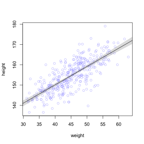
The posterior distribution gives rise to a set of lines for each possible values of $\alpha$, $\beta$. In the below plot, the shade is the 97% interval of posterior distribution of ${\mu }_i$ - sum of gaussians from $\alpha$, $\beta$, gives rise to a gaussian ${\mu }_i$ for every $w_i$.

$${\mu }_i=\alpha +\beta .(w_i-\bar{w})$$

Note that at $w_i=w$, the variability is smallest because it is just the posterior distribution of $\alpha$ which in turn is the posterior distribution of the average height in the population.

Recipe for creating posterior intervals for the model:

“Use link to generate distributions of posterior values for μ. The default behavior of link is to use the original data, so you have to pass it a list of new horizontal axis values you want to plot posterior predictions across. (2) Use summary functions like mean or PI to find averages and lower and upper bounds of μ for each value of the predictor variable. (3) Finally, use plotting functions like lines and shade to draw the lines and intervals. Or you might plot the distributions of the predictions, or do further numerical calculations with them. It’s really up to you. This recipe works for every model we fit in the book. As long as you know the structure of the model—how parameters relate to the data—you can use samples from the posterior to describe any aspect of the model’s behavior.” (McElreath, 2020, p. 107)

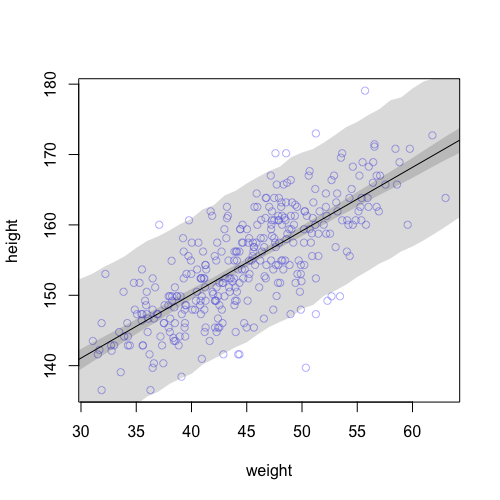
The predictive posterior distribution takes into account the unobserved variability modeled by $\sigma$ and provides a predictive window for the data points. In the below plot, the shade is the 97% predictive posterior of height.

“Rethinking: Two kinds of uncertainty. In the procedure above, we encountered both uncertainty in parameter values and uncertainty in a sampling process. These are distinct concepts, even though they are processed much the same way and end up blended together in the posterior predictive simulation. The posterior distribution is a ranking of the relative plausibilities of every possible combination of parameter values. The distribution of simulated outcomes, like height, is instead a distribution that includes sampling variation from some process that generates Gaussian random variables. This sampling variation is still a model assumption. It’s no more or less objective than the posterior distribution. Both kinds of uncertainty matter, at least sometimes. But it’s important to keep them straight, because they depend upon different model assumptions. Furthermore, it’s possible to view the Gaussian likelihood as a purely epistemological assumption (a device for estimating the mean and variance of a variable), rather than an ontological assumption about what future data will look like. In that case, it may not make complete sense to simulate outcomes.” (McElreath, 2020, p. 109)

Polynomial regression and B-splines

Polynomial regression

The idea is essentially the same as linear regression - expect we use higher order equations with quadratic and cubic terms.

Here is how a quadratic model would look like:

$$\begin{array}{rl}{h}_i& \sim Normal({\mu }_i,\sigma )\\ {\mu }_i& =\alpha +{\beta }_1.x_i+{\beta }_2.x_i^2\\ x_i& =\frac{w_i-\bar{w}}{{\sigma }_x}\end{array}$$

Here, $x_i$ is standardized weights - weights that have been mean subtracted and normalized by the standard deviation.

The problem is setting the priors. It is not clear what ${\beta }_2$ should be. The others can be the same as the linear model as the assumptions all apply. Intuitively, if we think of ${\beta }_2{x}_i^2$ term as an additional term that kicks in when $x_i$ becomes large and adds values to the line, positive ${\beta }_2$ will allow the polynomial to curve outward from the line (increase faster than the line) and negative would make the polynomial curve inward (decrease slower than the line). Based on the height data, ${\beta }_2$ should be negative, so we need to allow our constraints to be positive and negative.

$$\begin{array}{rl}\alpha & \sim Normal(178,20)\\ {\beta }_1& \sim Log-Normal(0,1)\\ {\beta }_2& \sim Normal(0,1)\\ \sigma & \sim Uniform(0,50)\end{array}$$

Video 03 notes:

Flow

I like the idea of flow described in the video lectures. Basically, learning should have some resistance that you can feel the flow of air/water against you as you are moving forward. But the learning barrier should not be so high that you stop moving forward (no flow) or so low that you don’t learn anything new (no flow) as you move forward. I converged on this idea independently but I love the framing of it and the independent confirmation. I want to incorporate this more often in my mentorship.

Generative models

• Dynamic - changes in weight and height based on growth pattern. gaussian variation is result of fluctuations in the growth pattern of the organism.
• Static - association between weight and height. gaussian variation is a function of growth history?

Static model:

flowchart LR
	H --> W
	U((U)) --> W 

Estimator

$E(W_i|H_i)=\alpha +\beta H_i$

$$Pr(\alpha ,\beta ,\sigma |H_i,W_i)=\frac{Pr(H_i,W_i|\alpha ,\beta ,\sigma )Pr(\alpha ,\beta ,\sigma )}{Z}$$

$Pr(H_i,W_i|\alpha ,\beta ,\sigma )$ - garden of forking. how many ways can we see the data for different values of $\alpha$, $\beta$, $\sigma$.
$Pr(\alpha ,\beta ,\sigma )$ - based on the previous data (or prior guess) how likely are different values of $\alpha$, $\beta$, $\sigma$.

The above bayesian estimation is written as:
$W_i\sim Normal({\mu }_i,\sigma )$
${\mu }_i=\alpha +\beta H_i$

Prior predictive distributions - used to figure out scientifically justifiable priors (there is no correct priors). Priors not important in simple models, but very important (useful) in complex models.

Statistical Interpretation:

• Parameters are not independent of one another - they cannot always be independently interpreted.
• Posterior predictions to interpret parameters.

POV: Linear regression are measurement devices. They measure socially constructive objects.

Generative models vs statistical models.

Video 04 notes:

Categorical variables

Unlike the books, the video lectures have flipped height and weight. Maybe I need to do that too, just for fun.

Adding categories - sex and its influence on height and weight.

flowchart LR
S --> H
S --> W
H --> W

The read out of DAGs is a direct cause, not indirect cause:

$$\begin{array}{rl}H& =f_H(S)\\ W& =f_W(H,S)\end{array}$$

There is always unmodeled and unobserved causes. Most of them are ignorable unless they are shared (as they might be confounds).

flowchart LR
S --> H
S --> W
H --> W
U((U)) --> H
V((V)) --> W
T((T)) --> S

Direct effect of Sex - simulating posterior and looking at the difference.

This is an interesting analysis and something to try about.

Polynomial

Polynomials are not very useful as they are sensitive to the whole datapoints and not local datapoints when the curvature is determined (this is same as linear fits when the slope and the intercept depends on a few outliners more). Hence polynomials are not preferred and splines are much preferred as they allow for local smoothening.

Because of this, we cannot make predictions outside the fitted region (no credibility).

Splines - very useful when there is not enough scientific information - use local information to make prediction by smoothing.

$${\mu }_i=\alpha +w_1{B}_{i,1}+w_1{B}_{i,2}+w_1{B}_{i,3}+...$$

The basis function dictates where the basis is non-zero and where it is zero. Basically how to break the axis down - anchor points - and how each basis changes between two anchor points. The weights add relative contributions of each of these basis functions.

This basic functions can be linear, can be quadratic, cubic splines etc.

Footnotes

Footnotes

1. This is based on the mean and the variance of a standard binomial distribution with two outcomes - 0 and 1. The mean is 0.5 ($np=0.5$ for $n=1$, $p=0.5$; binomial distribution) and variance 0.25 ($npq=0.25$ for $n=1$, $p=0.5$, $q=0.5$). If the outcomes were -0.5 and 0.5 (subtract the previous distribution with 0.5), the mean would be 0, but the variance would still be 0.25. If the outcomes were -1 and 1 (multiple the -0.5, 0.5 distribution with 2), the variance will have 4 multiplied to it (variance is squared difference between sample and mean), so the variance should be 1. ↩

2. I had a lot of trouble getting it working as I was initially doing sum and not average. When taking sum, the mean and the variance were $np$ and $npq$ respectively, which is the expected mean, variance for a sum of sequences from a binomial distribution. ↩